Visualize results
A good visualization can be a very powerful tool to understand the results of a simulation and to help to refine the design of an instrument or to see how a specific observation setup can be improved.
A 3 dimensional picture
Specifically when designing an instrument, we might want a 3-D rendering of the mirrors, detectors, and gratings as well as the photon path. We want to see where photons are absorbed and where they are scattered.
Depending on the target audience of the visualization (e.g. a detailed technical rendering for a publication, or a 3D display in a webpage) different output formats are required. marxs.visualization supports different backends for display and rendering with different display options. Not every backend supports every option and we welcome code contributions to improve the plotting.
Currently, the following plotting packages are supported:
X3D is an open XML-based standard to 3D models in the web-browser and can be displayed with different libraries. Importantly, it can also be rendered directly in a Jupyter notebook.
Mayavi is a Python package for interactive 3-D displays that uses VTK underneath. Using plotting routines from
marxs.visualization.mayaviscenes can be displayed right in the same Python session or jupyter notebook where the MARXS simulation is running or be exported as static images (e.g. PNG) or as X3D suitable for inclusion in a web page or AAS journal paper.three.js is a javascript package to render 3d content in a web-browser using WebGL technology. MARXS does not display this content directly, but outputs code (
marxs.visualization.threejs) or json formatted data (marxs.visualization.threejsjson) that can be included in a web page.
All backends support a function called plot_object which plots objects in the simulation such as apertures, mirrors, or detectors and a function called plot_rays which shows the path the photons have taken through the instrument in any specific simulation. In the example below, we use the mayavi backend to explain these functions. The arguments for these functions are very similar for all backends, but some differences are unavoidable. For example, marxs.visualization.mayavi.plot_rays needs a reference to the scene where the rays will be added, while marxs.visualization.threejs.plot_rays requires a file handle where relevant javascript commands can be written - see Reference/API for more details.
First, we need to set up mirrors, gratings and detectors (here gratings on a Rowland torus). The entrance aperture is just a thin ring, like the effective area of a single shell in a Wolter type-I telescope:
>>> from marxs import optics, design, analysis
>>> from marxs.design import rowland
>>> import astropy.units as u
>>> rowland = design.rowland.RowlandTorus(5000, 5000)
>>> aper = optics.CircleAperture(position=[12000, 0, 0],
...                              zoom=[1, 1000, 1000],
...                              r_inner=960)
>>> mirr = optics.FlatStack(position=[11000, 0, 0],
...                         zoom=[20, 1000, 1000],
...                         elements=[optics.PerfectLens,
...                         optics.RadialMirrorScatter],
...                         keywords = [{'focallength': 11000},
...                                     {'inplanescatter': 4 * u.arcsec,
...                                      'perpplanescatter': 0.6 * u.arcsec}])
In our figure, we want to color the diffraction gratings and the photons that pass through them. For this purpose we make a new class of grating that inherits from FlatGrating but additionally assigns a value to the colorid. The method specific_process_photons` is defined as part of `~marxs.optics.FlatOpticalElement` and it returns a dictionary of arrays that are assigned to the corresponding column in the ``photons table. Here, we simply add another column to that:
>>> class ColoredFlatGrating(optics.FlatGrating):
...     '''Flat grating that also assigns a color to all passing photons.'''
...     def specific_process_photons(self, *args, **kwargs):
...         out = super(ColoredFlatGrating, self).specific_process_photons(*args, **kwargs)
...         out['colorid'] = self.colorid if hasattr(self, 'colorid') else np.nan
...         return out
We place a set of transmission gratings below the mirror and add CCDs on the Rowland torus:
>>> gas = design.rowland.GratingArrayStructure(rowland=rowland, d_element=[180, 180],
...                                            radius=[870, 910],
...                                            elem_class=ColoredFlatGrating,
...                                            elem_args={'d': 2e-4, 'zoom': [1, 80, 80],
...                                                       'order_selector': optics.OrderSelector([-1, 0, 1])})
>>> det_kwargs = {'d_element': [105, 50], 'elem_class': optics.FlatDetector,
...               'elem_args': {'zoom': [1, 50, 20], 'pixsize': 0.01}}
>>> det = design.rowland.RectangularGrid(rowland=rowland, y_range=[-200, 200], **det_kwargs)
>>> projectfp = analysis.ProjectOntoPlane()
Each optical element in MARXS has some default values to customize its looks in its display property, which may or may not be used by the individual backend since not every backend supports the same display settings.
The most common settings are display['color'] (which can be any RGB tuple or any color valid in matplotlib) and display['opacity'] (a number between 0 and 1).
Usually, display is a class dictionary, so any change on any one object will affect all elements of that class:
>>> mirr.display['opacity'] = 0.5
>>> optics.FlatDetector.display['color'] = 'orange'
To change just one particular element we copy the class dictionary to that element and set the color. In this example, we calculate the angle that each grating has from the y-axis. We split that in three regions and color the gratings accordingly:
>>> import copy
>>> import numpy as np
>>> gratingcolors = 'bgr'
>>> for e in gas.elements:
...     e.display = copy.deepcopy(e.display)
...     e.ang = (np.arctan(e.pos4d[1,3] / e.pos4d[2, 3]) + np.pi/2) % (np.pi)
...     e.colorid = int(e.ang / np.pi * 3)
...     e.display['color'] = gratingcolors[e.colorid]
Using MARXS to visualize sub-aperturing
In this example, we use MARXS to explain how sub-aperturing works. Continuing the code from above, we define an instrument setup, run a simulation, and plot results both in 2d and in 3d. This is a fully functional ray-trace simulation; the only unrealistic point is the grating constant of the diffraction gratings which is about an order of magnitude smaller than current gratings.
2d plot
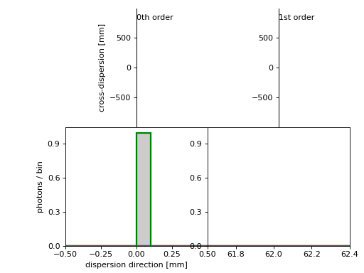
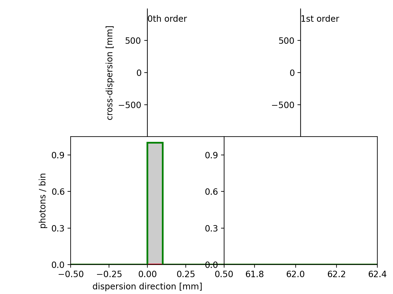
We want to know how photons that go through a particular set of gratings are distributed compared to the total point-spread function (PSF). Therefore, we assign a color to every sector of gratings and in our plots, we color gratings in this sector and photons that passed through it accordingly.
(Source code, png, hires.png, pdf)

On the plot, we see that photons from each sector (e.g. the sector that colors photons red) form a strip on the detector. Only adding up photons from all sectors gives us a round PSF. Subaperturing is the idea to disperse only photons from one sector, such that the PSF in cross-dispersion direction is large, but the dispersion in cross-dispersion direction is much smaller (the green sector in the figure). Thus, the spectral resolution of the dispersed spectrum will be higher than for a spectrograph that uses the full PSF. Note that the first order photons are asymmetrically distributed unlike the zeroth order. This is due to the finite sizes of the flat diffraction gratings that deviate from the curved Rowland torus. Based on this simulation, we can now decide to implement sub-aperturing in our instrument. We will instruct the engineers to mount ggratings only at the green colored positions so that we get a sharper line (a better resolving power) compared with using every photon that passes through the mirror.
3d output
Next, we want to show how the instrument that we use above looks in the 3d.
Very similar to the previous example, we combine mirror, detector, and grating into Sequence. We also define a marxs.simulator.KeepCol object, which we pass into our Sequence. When we call the Sequence, the KeepCol object will make a copy of a column (here the “pos” column) and store that.
Another change compared to the 2d plotting is that we generate a lot fewer photons because the lines indicating the photon paths can make the gratings hard to see in 3d if there are too many of them:
>>> import numpy as np
>>> from astropy.coordinates import SkyCoord
>>> import astropy.units as u
>>> from marxs import source, simulator
>>> # object to save intermediate photons positions after every step of the simulation
>>> pos = simulator.KeepCol('pos')
>>> instrum = simulator.Sequence(elements=[aper, mirr, gas, det, projectfp], postprocess_steps=[pos])
>>> star = source.PointSource(coords=SkyCoord(30., 30., unit='deg'))
>>> pointing = source.FixedPointing(coords=SkyCoord(30., 30., unit='deg'))
>>> photons = star.generate_photons(100 * u.s)
>>> photons = pointing(photons)
>>> photons = instrum(photons)
>>> ind = (photons['probability'] > 0) & (photons['facet'] >=0)
>>> posdat = pos.format_positions()[ind, :, :]
First, plot the objects that make up the instrument (aperture, mirror, gratings, detectors):
.. doctest-requires:: mayavi
>>> from mayavi import mlab
>>> from marxs.visualization.mayavi import plot_object, plot_rays
>>> fig = mlab.figure(bgcolor=(1,1,1))
>>> obj = plot_object(instrum, viewer=fig)
Now, we plot the rays using their colorid and a global color map that matches the blue-red values that we assigned to the gratings already:
.. doctest-requires:: mayavi
>>> rays = plot_rays(posdat, scalar=photons['colorid'][ind],
...                  kwargssurface={'opacity': .5,
...                                 'line_width': 1,
...                                  'colormap': 'blue-red'})
MARXS can also display non-physical objects. The following code will add a fraction of the Rowland torus:
.. doctest-requires:: mayavi
>>> rowland.display['coo2'] = np.linspace(-.2, .2, 60)
>>> obj = plot_object(rowland, viewer=fig)
3D view of the instrument set up. Lines are photon paths. All detectors are orange, and the gratings are red, green, and blue, depending on their position. The mirror and the aperture are shown with their default representation (white box and transparent green plate with the aperture hole). Part of the Rowland torus is shown as a red surface. Use your mouse to rotate, pan and zoom. (Detailed instructions for camera navigation).
Reference/API
marxs.visualization Package
MARXS supports several backends for 3D plotting; each of which is implemented as a submodule.
To plot using a specific backend, import the relevant submodule.
Classes
|
Configuration parameters for my subpackage. |
Class Inheritance Diagram
marxs.visualization.x3d Module
X3D plotting backend
X3D is an open standard for interactive 3D models on the Web. X3D models are stored in XML files and can be viewed in the Jupyter notebook or on the web with different js libraries without the installation of a plug-in.
This module implements the Scene
class, which can represent itself as a complete HTML page to be
rendered directly or it can return the XML format to be saved
and used in other contexts.
Each plotting routine requires a Scene
as input and objects are added to it (if no scene is passed in,
an empty one is generated.)
Under the hood, the XML is constructed using the x3d Python package.
Functions
|
|
|
Plot a set of triangles. |
|
Plot a parametric surface. |
|
Plot a plane, e.g. an aperture with an inner hole. |
|
Plot a rectangular box for an object. |
|
Recursively plot objects contained in a container. |
|
Plot any marxs object with using X3D as a backend. |
|
Plot lines for simulated rays. |
Classes
|
X3D Scene with added _repr_html_ for notebook output |
Class Inheritance Diagram
marxs.visualization.mayavi Module
Mayavi plotting backend
Mayavi is a python package for interactive 3-D displays that uses VTK
underneath. Functions in this module display rays or objects in 3D
using mayavi. Each of them requires a mayavi.core.scene.Scene
instance as input and returns a mayavi object (or a list of those),
e.g. a mayavi.visual.Box instance.
The plotting routines attempt to find all valid OpenGL properties by
name in the display dictionaries and apply those to the plotted
object.
Functions
|
Plot a rectangular box for an object. |
|
Recursively plot objects contained in a container. |
|
Plot a cylinder for an object. |
|
Plot any marxs object with using Mayavi as a backend. |
|
Plot lines for simulated rays. |
|
Plot a parametric surface. |
|
Plot a plane with an inner hole such as an aperture. |
marxs.visualization.threejs Module
Plot routines for display with three.js.
Each routine adds strings to a file and thus each routing requires a writable file object as an argument. This file can then be included in a webpage that loads the three.js javascript package.
Note that routine to display a torus is modified relative to the official three.js release to allow more parameters; the modified version is included in the MARXS source code. Also, note that the output file is not a valid webside by itself. Instead, it is a list of javascript commands, that needs to be included into a website after the nesessary setup and package loading.
Functions
|
Flatten array and return string representation for insertion into js. |
|
Output three.js commands to include a box-shaped optical element. |
|
Recursivey output three.js commands to print all elements of a container. |
|
Construct a string that can be pasted into a javascript template to describe a three.js material. |
|
Construct a string that can be pasted into a javascript template to describe a three.js material. |
|
Plot any MARXS object with three.js as backend. |
|
Plot lines for simulated rays. |
|
Output commands to display (part of) a torus. |
|
Output commands for a plane with an inner hole. |
marxs.visualization.threejsjson Module
Plot routines for json output to be loaded into three.js.
Each routine returns a json dictionary. These json dictionaries can be collected in
a list and written to a file with write, which
checks the formatting and adds metadata.
Just as threejs this backend provides input for a webpage that
will then use the three.js library to render the 3D model. The main
difference is that threejs outputs plain text for each object,
while the json written by this module is much smaller if the model contains many copies
of the same object (e.g. hundreds of diffraction gratings). Also, the json data can be
updated with no changes necessary to the html page.
MARXS includes loader.html as an example how MARXSloader.js (included in MARXS
as well) can be used to load the json file and construct the three.js objects.
Note that routine to display a torus is modified relative to the official three.js release to allow more parameters, the modified version is included in MARXS.
For reference, here is a short summary of the json data layout.
There are two main entries: metadata (a list with the MARXS version, writer, etc…)
and objects which is a list of lists.
Each of the sublists has the following fields:
n: number of objects in listname: string or list (if there are sevaral object in this sublist)material: stringmaterialpropterties: dictgeometry: type (e.g.BufferGeometry, see three.js)if
geometryis a buffer Geometry:pos,color(lists of numbers)otherwise: -
pos4d: list of lists of 16 numbers -geometrypars: list (meaning depends on geometry, e.g. radius of torus)
Functions
|
Describe a box-shaped optical elements. |
|
'Recursively output three.js json to describe all elements of a container. |
|
'Format any MARXS object as a json string. |
|
Plot lines for simulated rays. |
|
Describe a (possibly incomplete) torus. |
|
Describe a plane with a hole, such as an aperture of baffle. |
|
Add metadata and write json for three.js to disk |
marxs.visualization.utils Module
This module collects helper functions for visualization backends.
The functions here are not intended to be called directly by the user. Instead, they refractor common tasks that are used in several visualization backends.
Functions
|
Convert color tuple to hex string. |
|
Combine two disjoint triangulations into one set of points |
|
Look for color information in dictionary. |
|
Return printable name for objects or functions. |
|
|
|
Triangulation of a plane with an inner hole |
|
Look up a plotting routine for an object and execute it. |
Classes
|
A dictionary to store how an element is displayed in plotting. |
Warning class for MARXS objects missing from plotting |