Coordinates, physical units and polarization
Coordinate system
Marxs employs a Cartesian coordinate system. All optical elements can be freely placed at any position and any angle in this space, but we recommend the following conventions for simplicity (examples and predefined missions in this package follow those conventions as far as possible):
The optical axis of the telescope coincides with the x-axis. A source on the optical axis is at \(x=+\infty\) and photons travel towards the origin.
The origin of the coordinate system is at the telescope focus.
The y-axis coincides with the dispersion direction of gratings.
Marxs uses homogeneous coordinates, which describe position and direction in a 4 dimensional coordinate space, for example \([3, 0, 0, 1]\) describes a point at x=3, y=0 and z=0; \([3, 0, 0, 0]\) describes the vector from the origin to that point. Homogeneous coordinates have one important advantage compared with a normal 3-d description of Euclidean space: In homogeneous coordinates, rotation, zoom, and translations together can be described by a \([4, 4]\) matrix and several of these operations can be chained simply by multiplying the matrices.
Every optical element in marxs (and some other objects, too) has such a \([4, 4]\) matrix
associated with it in an attribute called element.pos4d.
All optical elements have some default location and position. Typically, their active surface (e.g.
the surface of a mirror or detector) is in the y-z plane. The center is at the origin of the
coordinate system and the default size in each dimension is 1, measured from the center.
Thus, e.g. the default definition for a marxs.optics.detector.FlatDetector, makes a detector surface with
the following corners (in 3-d x,y,z coordinates): [0, -1, -1], [0, -1, 1], [0,
1, 1] and [0, 1, -1].
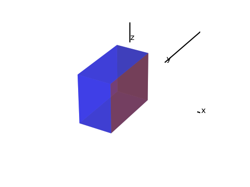
Note that in a 3D visualization (see Visualize results), some elements might be shown with a thickness
2 (from \(x=-1\) to \(x=+1\)), so that the “active surface” is in the middle of a box,
while others might show the “active surface” as the edge of the box as in the
sketch below. Details depend on the capabilities of the plotting backend
(backends and options are listed in Reference/API).
However, when running the ray-trace the code calculates the intersection with the “active surface” in the y-z plane independent of the thickness in x-direction. There are exceptions to these defaults, those are noted in the description of the individual optical elements. See the following sketch, where the “active surface” is shown in red:

In order to place elements in the experiment, the optical element needs to be scaled (zoomed), rotated and translated to the new position. There are two ways to specify that:
Pass a \([4,4]\) matrix to the optical element:
>>> import numpy as np
>>> from marxs.optics import Baffle
>>> pos4d = np.array([[1., 0., 0., 5.],
...                   [0., 2., 0., 0.],
...                   [0., 0., 2., 0.],
...                   [0., 0., 0., 1.]])
>>> baf1 = Baffle(pos4d=pos4d)
This sides of this baffle have length 4 (from -2 to 2). The center is on the x-axis, but 5 units upwards from the origin.
Use the keywords
orientation,zoom, andposition. The code will construct thepos4dmatrix from those keywords, by first scaling withzoom, then applying the rotation matrixorientationand lastly, moving the center of the optical element toposition. The same baffle as above can also be written as:>>> baf2 = Baffle(zoom=[1., 2., 2.], position=[5., 0., 0.]) >>> np.all(baf2.pos4d == baf1.pos4d) np.True_
It is an error to specify
pos4dand any of theorientation,zoom, andpositionkeywords at the same time.
Note
The transforms3d package provides several functions to calculate 3-d and 4-d matrices from Euler angles, axis and angle, quaternions and several other representations. This package is installed together with marxs.
Polarization
In principle, MARXS supports polarization ray-tracing, but only very few optical elements actually change the polarization vector of a photon. In these cases, that is explicitly explained in the description. All other elements do not change the polarization state of a photon. For some, this is physically correct (e.g. a photon passing through the hole in baffle), in other cases this behavior just a reasonable approximation (e.g. most diffraction gratings polarize light only to a very small degree).
Make sure to inspect the implementation of all relevant optical elements if your simulation makes use of the photon polarization vector.
In the ray-trace itself, MARXS represents the polarization of each photon as a 3d-vector and then uses matrices to move this vector in space. This is an extension of the 2-d Jones calculus, which is particularly suited for light paths that are not all parallel to an optical bench [Chipman_1992] . See [Yun_et_al_2011] and [Yun_2011] for details on polarization ray tracing and the derivation of the relevant matrices.
This mechanism can handle both linear and circular polarized light. However, the light sources currently included in MARXS only support linear polarization.
Bibliography
Physical units
MARXS uses astropy units and
astropy.coordinates.SkyCoord for input of source properties and
coordinates. This makes quantities having a specific unit and avoids confusion
between degree and radian, eV and keV and so on.
Internally, however, this extra unit makes the computation too slow. Thus, all properties are converted to float using the following conventions:
Length: base unit is mm.
Energy: base unit is keV.
Angles: Always expressed in radian.
When designing an instrument, these units must be used.