Visualize results
A good visualization can be a very powerful tool to understand the results of a simulation and to help to refine the design of an instrument or to see how a specific observation setup can be improved.
A 3 dimensional picture
Specifically when designing an instrument, we might want a 3-D rendering of the mirrors, detectors, and gratings as well as the photon path. We want to see where photons are absorbed and where they are scattered.
Depending on the target audience of the visualization (e.g. a detailed technical rendering for a publication, or a 3D display in a webpage) different output formats are required. marxs.visualization supports different backends for display and rendering with different display options. Not every backend supports every option and we welcome code contributions to improve the plotting.
Currently, the following plotting packages are supported:
X3D is an open XML-based standard to 3D models in the web-browser and can be displayed with different libraries. Importantly, it can also be rendered directly in a Jupyter notebook.
three.js is a javascript package to render 3d content in a web-browser using WebGL technology. MARXS does not display this content directly, but outputs code (
marxs.visualization.threejs) or json formatted data (marxs.visualization.threejsjson) that can be included in a web page.
All backends support a function called plot_object which plots objects in the simulation such as apertures, mirrors, or detectors and a function called plot_rays which shows the path the photons have taken through the instrument in any specific simulation. In the example below, we use the x3d backend to explain these functions. The arguments for these functions are very similar for all backends, but some differences are unavoidable. For example, marxs.visualization.x3d.plot_rays needs a reference to the scene where the rays will be added, while marxs.visualization.threejs.plot_rays requires a file handle where relevant javascript commands can be written - see Reference/API for more details.
First, we need to set up mirrors, gratings and detectors (here gratings on a Rowland torus). The entrance aperture is just a thin ring, like the effective area of a single shell in a Wolter type-I telescope:
from marxs import optics, design, analysis
from marxs.design import rowland
import astropy.units as u
rowland = design.rowland.RowlandTorus(5000, 5000)
aper = optics.CircleAperture(position=[12000, 0, 0],
                              zoom=[1, 1000, 1000],
                              r_inner=960)
mirr = optics.FlatStack(position=[11000, 0, 0],
                        zoom=[20, 1000, 1000],
                        elements=[optics.PerfectLens,
                                  optics.RadialMirrorScatter],
                        keywords = [{'focallength': 11000},
                                    {'inplanescatter': 4 * u.arcsec,
                                     'perpplanescatter': 0.6 * u.arcsec}])
In our figure, we want to color the diffraction gratings and the photons that pass through them. For this purpose we make a new class of grating that inherits from FlatGrating but additionally assigns a value to the colorid. The method specific_process_photons is defined as part of FlatOpticalElement and it returns a dictionary of arrays that are assigned to the corresponding column in the photons table. Here, we simply add another column to that:
class ColoredFlatGrating(optics.FlatGrating):
    '''Flat grating that also assigns a color to all passing photons.'''
    def specific_process_photons(self, *args, **kwargs):
        out = super().specific_process_photons(*args, **kwargs)
        out['colorid'] = self.colorid if hasattr(self, 'colorid') else np.nan
        return out
We place a set of transmission gratings below the mirror and add CCDs on the Rowland torus:
gas = design.rowland.GratingArrayStructure(rowland=rowland,
      d_element=[180, 180],
      radius=[870, 910],
      elem_class=ColoredFlatGrating,
      elem_args={'d': 2e-4, 'zoom': [1, 70, 70],
                 'order_selector': optics.OrderSelector([-1, 0, 1])})
det_kwargs = {'d_element': [105, 50], 'elem_class': optics.FlatDetector,
             'elem_args': {'zoom': [1, 50, 20], 'pixsize': 0.01}}
det = design.rowland.RectangularGrid(rowland=rowland, y_range=[-210, 200],
                                     guess_distance=0, **det_kwargs)
projectfp = analysis.ProjectOntoPlane()
Each optical element in MARXS has some default values to customize its looks in its display property, which may or may not be used by the individual backend since not every backend supports the same display settings.
The most common settings are display['color'] (which can be any RGB tuple or any color valid in matplotlib) and display['opacity'] (a number between 0 and 1).
Usually, display is a class dictionary, so any change on any one object will affect all elements of that class:
mirr.display['opacity'] = 0.5
optics.FlatDetector.display['color'] = 'orange'
To change just one particular element we copy the class dictionary to that element and set the color. In this example, we calculate the angle that each grating has from the y-axis. We split that in three regions and color the gratings accordingly:
import copy
import numpy as np

gratingcolors = ['blue', 'green', 'red']
for e in gas.elements:
    e.display = copy.deepcopy(e.display)
    e.ang = (np.arctan(e.pos4d[1,3] / e.pos4d[2, 3]) + np.pi/2) % (np.pi)
    e.colorid = int(e.ang / np.pi * 3)
    e.display['color'] = gratingcolors[e.colorid]
Using MARXS to visualize sub-aperturing
In this example, we use MARXS to explain how sub-aperturing works. Continuing the code from above, we define an instrument setup, run a simulation, and plot results both in 2d and in 3d. This is a fully functional ray-trace simulation; the only unrealistic point is the grating constant of the diffraction gratings which is about an order of magnitude smaller than current gratings.
2d plot
We want to know how photons that go through a particular set of gratings are distributed compared to the total point-spread function (PSF). Therefore, we assign a color to every sector of gratings and in our plots, we color gratings in this sector and photons that passed through it accordingly.
(Source code, png, hires.png, pdf)
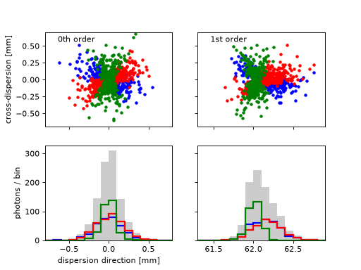
On the plot, we see that photons from each sector (e.g. the sector that colors photons red) form a strip on the detector. Only adding up photons from all sectors gives us a round PSF. Subaperturing is the idea to disperse only photons from one sector, such that the PSF in cross-dispersion direction is large, but the dispersion in cross-dispersion direction is much smaller (the green sector in the figure). Thus, the spectral resolution of the dispersed spectrum will be higher than for a spectrograph that uses the full PSF. Note that the first order photons are asymmetrically distributed unlike the zeroth order. This is due to the finite sizes of the flat diffraction gratings that deviate from the curved Rowland torus. Based on this simulation, we can now decide to implement sub-aperturing in our instrument. We will instruct the engineers to mount gratings only at the green colored positions so that we get a sharper line (a better resolving power) compared with using every photon that passes through the mirror.
3d output
Next, we want to show how the instrument that we use above looks in the 3d.
Very similar to the previous example, we combine mirror, detector, and grating into Sequence. We also define a marxs.simulator.KeepCol object, which we pass into our Sequence. When we call the Sequence, the KeepCol object will make a copy of a column (here the “pos” column) and store that.
Another change compared to the 2d plotting is that we generate a lot fewer photons because the lines indicating the photon paths can make the gratings hard to see in 3d if there are too many of them:
ind = (photons['probability'] > 0) & np.isfinite(photons['colorid'])
posdat = pos.format_positions()[ind, :, :]
First, plot the objects that make up the instrument (aperture, mirror, gratings, detectors):
from marxs.visualization.x3d import plot_object, plot_rays
scene = plot_object(instrum)
Now, we create a matplotlib colormap that matches the colors we chose for the gratings and then plot the rays using their colorid:
import matplotlib as mpl
cmap = mpl.colors.ListedColormap(gratingcolors)
scene = plot_rays(posdat, scalar=photons['colorid'][ind], cmap=cmap, scene=scene)
MARXS can also display non-physical objects. The following code will add a fraction of the Rowland torus. We modify the default display settings to show the torus parameterized with more points so that we get a smoother surface:
rowland.display['coo1'] = np.linspace(0, 2 * np.pi + 0.01, 600)
rowland.display['coo2'] = np.linspace(-.2, .2, 60)
scene = plot_object(rowland, scene=scene)
At last, we set a light background and save the scene to an X3D file that we include into these documentation web pages for interactive viewing.
import x3d
scene.children.append(
     x3d.Background(skyColor=[(0.9, 0.9, 0.9)])
   )
with open('_static/ex_vis.x3d', 'w') as f:
    f.write(scene.embed_in_X3D().XML())
3D view of the instrument set up. Lines are photon paths. All detectors are orange, and the gratings are red, green, and blue, depending on their position. The mirror and the aperture are shown with their default representation (white box and transparent green plate with the aperture hole). Part of the Rowland torus is shown as a red surface. Use your mouse to rotate, pan and zoom; double click to set the center of rotation. The default viewing position is centered on (0, 0, 0) with some optical elements outside of the field of view. (Detailed instructions for camera navigation).