Estimating tolerances requirements
A common problem when designing an instrument is to estimate how much the performance degrades with increasing misalignments. Detailed alignment work costs time and money, in particular if the alignment has to be done under X-rays and in vacuum. It is much cheaper if the alignment tolerances are loose and machining a surface is precice enough.
There are different degrees of freedom to consider. Each element can be moved in space in 6 ways, rotation around all three principal axes and translation along all three principal axes. Usually, misalignment will lead to reduced performance, e.g. because a mirror covers only part of the beam or because a detector is not located at the focus position any longer. In addition to positional uncertainties, some elements have other parameters that effect the perfomance in much the same way as misalignment does. For example, for dispersion gratings the grating period could differ a little from the specificed value. MARXS provides tools to help with the tolerancing process.
Test different misalignment values and energies
Tolerances can be estimated “by hand” by modifying the position and orientation
of one or more elements. The process is simple - one just has to modify the pos4d matrix (see Coordinate system) - but tedious if it needs to be done often. This module provides two functions to loop over a set of input values:
Both take an instrument definition, a function to vary parameters for some element, a list of of parameter values that shall be simulated, and a function to analyse the results for each simulation.
The first, run_tolerances works with an input photon list and runs one simulation for each dictionary of parameters values in the input. The second, run_tolerances_for_energies, iterates over photon energies and loops over run_tolerances for every energy.
run_tolerances has the following calling signature:
>>> out = run_tolerances(photons_in, instrum, wigglefunc, wiggleparts,
...                      parameters, analyzefunc)
We will now explain each of these parameters in more detail.
Photon list and definition of the instrument
The instrum is the instrument that will be analysed. This will
typically be a marxs.simulator.Sequence. It can contain
the entire instrument or only part of it. photons_in is a photon
list. If instrum contains all elements of the instrument, then
photons_in is simply a list of photons from any
source. Alternatively, photons_in can be processed through the
first few elements already, and instrum only contains the
remaining elements. For example, to determine the misalignments
for the detector, it might make sense to process the photons through
all upstream parts and then list only the detector in instrum.
Wiggle functions
This function changes the properties of one or more element in
instrum. The particular element or a list of elements is given as
wiggleparts parameter; the wiggleparts should also be part of
instrum or the wiggled parameters won’t affect the photon
propagation. The format of the wigglefunc is a function that
accepts an optical element (given in wiggleparts) and some
parameters (given in parameters, see below). This can function
modifies one or more elements based on the parameters. Users can write
any wigglefunc they need. Some common examples for wiggle
functions are part of this module:
wiggle
moveglobal
moveindividual
varyperiod
varyorderselector
varyattribute
Wiggle parameters
The parameters simply take the form of lists of dictionaries, where each dictionary contains the parameters for a single call of wigglefunc. These parameters are also propagated to the output.
As an example, varyperiod changes the period of one or more dispersion gratings, drawing values from a Gaussian distribution. A possible input could be:
>>> wigglepars = [{'period_mean': 0.0002, 'period_sigma': 1e-6},
...               {'period_mean': 0.0003, 'period_sigma': 1e-6},
...               {'period_mean': 0.0004, 'period_sigma': 1e-6},
...               {'period_mean': 0.0005, 'period_sigma': 1e-6}]
One common case is to move elements around in 6 degrees of freedom (translations in x,y,z and rotations around x,y,z), one degree of freedome at a time. Such a list can be build up with generate_6d_wigglelist.
Measure simulation results
For each simulation, we need to measure the result in some way, e.g. effective area and resolving power. Any function that accepts a photon list and returns a dictionary with resulting values will do:
>>> def get_PSF_width(photons):
...     return {'sy': np.std(photons['dety']), 'sx': np.std(photons['detx'])}
For the analysis of instruments with dispersion gratings, MARXS
provides CaptureResAeff which can be
initialized with some parameters such as the grating orders that
matter. The result is an object that can be called just like a
function:
>>> import astropy.units as u
>>> from marxs.analysis.gratings import CaptureResAeff
>>> resaeff = CaptureResAeff(A_geom=155 * u.cm**2,
...                          orders=[-1, 0, 1], dispersion_coord='tdetx')
Quick-look plotting
The result of a series of simulations is stored in an
astropy.table.Table. Typically,
run_tolerances or
run_tolerances_for_energies is run in a
separate script because it can take hours or even days to simulate
mislignments with many steps for all elements on an instrument. That
script would save results to a file (possibly after removing some
unwanted columns from the table).
That is why the quick-look plotting tools in this module assume that the data is stored in a file.
>>> from marxs.design.tolerancing import DispersedWigglePlotter()
>>> plotter = DispersedWigglePlotter()
>>> tab, fig = plotter.load_and_plot('file.fits', ['dx', 'dy', 'dz', 'rx', 'ry', 'rz'])
Differences for run_tolerances_for_energies
With run_tolerances_for_energies
simulations are run for different energies. Unlike
run_tolerances is it thus not enough to
put in a list of photons that already have passed some of the elements
in this instrument. For example, rays of different energy are
reflected differently in a mirror. Instead of a photon list,
run_tolerances_for_energies takes a photon
source and changes the energy for that source in eahc step. This only
works if the source is defined for monochromatic photons! Then, the
function takes the definitions of the instrument chopped into two
parts. The first part, contains all elements upsteam of the
gratingselements that are wiggled. These elements do not vary and
photons have to pass through them only once. The second part, contains
all downsteam elements starting with the elements that
varies. These elements need to be simulated again for every single
step.
Suggested modelling approach
In a real instrument, there is misalignment on all degrees of freedom at the same time but. a study of the complete parameter space is usually not computationally feasible. If there are only four elements, each with six degrees of freedom (dof), and we want to simulated just 10 steps for each dof, we would need \(10^{4*6}\) simulations. Fortunately, such a study is usually not required. Instead, MARXS provides tools to vary one (or a few) degree(s) of freedom at a time to understand how important each of them is. In practice, many dofs do not matter, because their alignment tolerances are loose. For example, if a circular mirror is rotated around its axis, the result will be the same. Another example is a detector that is larger than the image that the optics produce. If this detector is moved around a bit, it will still catch all photons.
So, we suggest running simulations for one dof at a time and decide on the maximal alignment tolerance for each dof. Then, decide on an alignment budget that assigns a tolerance to each dof. It’s easy for those dof where the requirements are loose, for those where the requirements are close to what is technically feasible, this needs some judgement calls: Which element is easiest to calibrate? Which can be manufactured best? Which has the best probability of delivering tighter margins, freeing up some room in the total error budget for other elements?
Once this error budget has been build up, as a second step, build up an instrument model where all dof are varied at the same time with the numbers from the eror budget. Run ray-traces with several (e.g. 1000) realizations of this model and see what fraction of the ray-traces fullfills the requirements on e.g. PSF size, spectral resolving power, or effective area.
Example: The Chandra HETG
Let’s look at an example of tolerancing for a single element. We simulate the Chandra/HETG instruments. The HETG consists of a few hundred grating facets, hel in place by a support structure (HESS). This HESS can swing in and out of the beam around a hinge. In this example, we study what happens if the entire HESS with all gratings is translated or rotated around the hinge.
We make a few simplifications compared to the real Chandra to simplify and speed up the simulations. First, the do not use the LissajousDither pattern, but just assume a fixed pointing. This simulation is not about pointing stability or dother patters, it’s about the HESS. Similarly, we assume a detector with infinite spatial resolution. With dither and sub-pixel repositioning the real accuracy in Chandra is already better than the size of the PSF, so that’s OK:
>>> import astropy.units as u
>>> from astropy.coordinates import SkyCoord
>>> from marxs.source import PointSource, FixedPointing
>>> from marxs.missions import chandra
>>> coords = SkyCoord(278. * u.deg, -77. * u.deg)
>>> src = PointSource(coords=coords)
>>> pnt = FixedPointing(coords=coords)
Define the elements that Chandra is made of:
>>> aper = chandra.Aperture()
>>> hrma = chandra.HRMA()
>>> hetg = chandra.HETG()
>>> acis = chandra.ACIS(chips=[4,5,6,7,8,9], aimpoint=chandra.AIMPOINTS['ACIS-S'])
We want to concentrate on the first diffration order. To speed up the computation, we tweka the grating efficiency such that the vast majority of photons ends up in either order -1 or +1. This will lead to an effective area that is far larger than in reality, but the relative change of effective area is still the same, i.e. if a misalignment of x mm leads to a 10% loss of effective area, that should still be true. We just get there much faster because we do not have to simulate as many source photons to build up sufficient signal. Such a cheat may not be acceptable in all situations, but since we might be running hundreds or thousands of simulations it’s worthwhile to think about ways to speed them up:
>>> from marxs.optics.grating import OrderSelector
>>> from marxs.missions import chandra
>>> hetg = chandra.HETG()
>>> selector = OrderSelector([-1, 0, 1], p=[.45, .1, .45])
>>> for e in hetg.elements:
...     e.order_selector = selector
The HETG has two parts with different grating constants and spectral traces on the detector. Our algorithm to measure the performance will be confused if there is more than one +1 order spot. We could either modify that algorithm, or, if we want to go with tools provided by MARXS, we can mask out all photons going through the HEG, so that only the HEG is left:
>>> def onlyHEG(photons):
...     photons['probability'][photons['mirror_shell'] < 2] = 0
...     return photons
Then, we import from the marxs.design.tolerancing module:
>>> from marxs.design.tolerancing import (moveglobal, run_tolerances_for_energies,
...                                       generate_6d_wigglelist)
>>> from marxs.analysis.gratings import CaptureResAeff
Next, we generate input for the function that will move the HESS around in our simulation. We do seven steps for every translation direction (-15, -5, -1, 0, 1, 5 and 15 mm) and nine teps for every rotation:
>>> changeglobal, changeind = generate_6d_wigglelist([0., 1., 5., 15.] * u.mm,
...                                                  [0., 1., 5., 10., 30.] * u.arcmin)
>>> resaeff = CaptureResAeff(A_geom=aper.area.to(u.cm**2), orders=[-1, 0, 1], dispersion_coord='tdetx')
So, let’s run it:
>>> from marxs.simulator import Sequence
>>> res = run_tolerances_for_energies(src, [1.5, 4.] * u.keV,
...                                   Sequence(elements=[pnt, aper, hrma, onlyMEG]),
...                                   Sequence(elements=[hetg, acis]),
...                                   moveglobal, hetg,
...                                   changeglobal,
...                                   resaeff,
...                                   t_source=10000)
- We save the results in a file named
wiggle_global.fitsand then make a quick-look plot. We use normal
matplotlib.pyplotcommands to modify the plot appearance slightly.
from marxs.design.tolerancing import DispersedWigglePlotter

# In this example, we use a file that's included in MARXS for test purposes
from astropy.utils.data import get_pkg_data_filename
filename = get_pkg_data_filename('data/wiggle_global.fits', 'marxs.design.tests')

wiggle_plotter = DispersedWigglePlotter()
tab, fig = wiggle_plotter.load_and_plot(filename, ['dx', 'dy', 'dz', 'rx', 'ry', 'rz'])

fig.axes[0].legend()

for i in range(6):
    fig.axes[2 * i].set_ylim([0, 1e3])
    fig.axes[2 * i + 1].set_ylim([0, 70])

fig.set_size_inches(8, 6)
fig.subplots_adjust(left=.09, right=.93, top=.95, wspace=1.)
(Source code, png, hires.png, pdf)
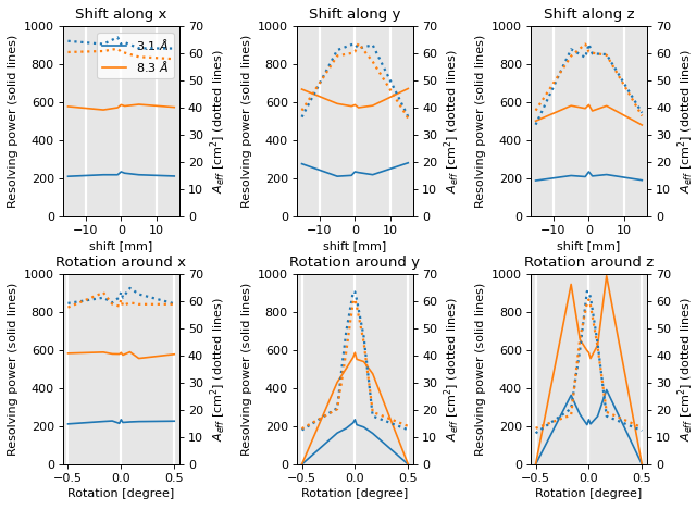
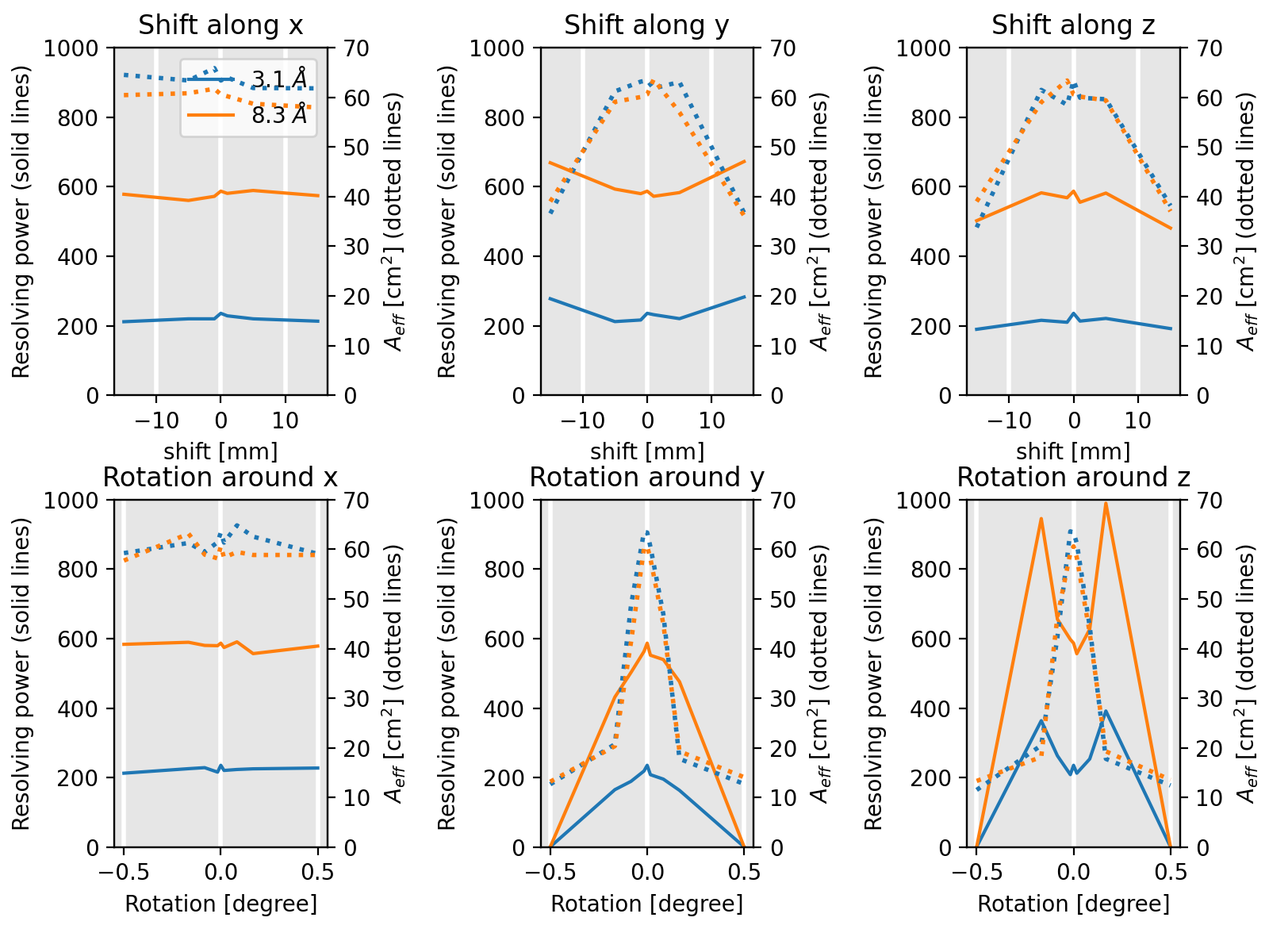

Looking at the plots we see the shifting the whole HETG by a few mm in any direction does not change the effective area or resolving power significantly. The rings of photons coming from the mirror is very narrow, in fact much narrower than the size of the grating facets. So shifting the HETG a little just means that the photons hit a different part of the grating. A shift in x is a focus change, but as long as all gratings are moved the same way, this has little impact. Similarly, a rotation around x just moves the position of the diffracted photons on the detector. As long as the rotation is small and the photons do not miss the detector, there is not much change. However, rotation around y, the dispersion direction, reduces the resolving power because some grating facets get defocussed with respect to the others. It also reduces the effective area because some gratings are moved out of the beam. Rotations around z are similar except that in this case the resolving power increases, because the gratings that normally cause the largest aberrations are removed form the beam.
Reference / API
marxs.design.tolerancing Module
Functions
|
Decorator for functions that modify optical elements. |
|
Move and rotate elements around principal axes. |
|
Move and rotate origin of the whole |
|
Move and rotate all elements of |
|
Move and rotate a marxs element around principal axes. |
|
Randomly draw different grating periods for different gratings |
|
Modify the OrderSelector for a grating |
|
Modify the attributes of an element. |
|
Run tolerancing calculations for a range of parameters |
|
Run tolerancing for a grid of parameters and energies |
|
Generate a list of parameters for the wiggle functions in this module. |
|
Select subset of tolerancing table with changes in 1 dof only |
Classes
Object to plot results of tolerancing simulations |
|
A wiggle plotter for gratings |