Further examples¶

In Visualize results we walked through one example where we defined an instrument setup, run photons through it, and looked at the results. In this section, we show another example.

Polarization¶

This is a laboratory setup. The X-ray source is some cathode, which we approximate as a monoenergetic point source (but see Specify flux, energy and polarization for a source for how to specify the whole spectrum). The aperture of the source is a small circular hole, so we simulate a beam of X-rays with a small opening angle:

from copy import copy
from transforms3d import euler
from marxs.source import LabPointSourceCone

from marxs.simulator import Sequence, KeepCol
light = LabPointSourceCone(position=[200., 0., 0.], direction=[-1., 0, 0],
                           half_opening=0.02)
# keep a copy of the position and direction for later
light_pos = light.position.copy()
light_dir = light.dir.copy()

These X-rays shine on a mirror (green rectangle in the figure below) at an angle very close to the Brewster angle, where only photons that are s-polarized (perpendicular to the plane of reflection, s from German senkrecht) are reflected:

import numpy as np
from marxs.optics import FlatBrewsterMirror, FlatDetector
rot1 = np.array([[2.**(-0.5), 0, -2.**(-0.5)],
                 [0, 1., 0],
                 [2.**(-0.5), 0, 2.**(-0.5)]])
m1 = FlatBrewsterMirror(orientation=rot1,zoom=[1, 10, 30])
# Keep a copy of the initial position for later
m1pos4d = m1.pos4d.copy()

Although the beam is slightly diverging, we will make the approximation that all photons hit the mirror at exactly the Brewster angle. Multi-layer mirrors with several hundred layers reach a reflection efficiency of a few percent for soft X-rays, where the wavelength of the photons that are reflected is fixed by the thickness of the layers and Bragg’s law. In this calculation, the reflection probability will have the same effect on every photon, so it just adds an overall normalization when we look at the number of photons detected later and we ignore it for now. Altogether, the combination of source and first mirror can be thought of as a “source of polarized X-rays”.

From the first mirror, the photons travel to a second mirror (blue), which reflects them onto a detector (yellow). Again, the mirror only reflects photons that are s-polarized and sends them to the detector:

rot2 = np.array([[2.**(-0.5), 0, 2.**(-0.5)],
                 [0, 1., 0],
                 [-2.**(-0.5), 0, 2.**(-0.5)]])
m2 = FlatBrewsterMirror(orientation=rot2,zoom=[1, 10, 30], position=[0, 0, 2e2])
# display is usually set for all objects of a class.
# To change only one mirror, make a copy of this dictionary first.
m2.display = copy(m2.display)
m2.display['color'] = 'blue'
det = FlatDetector(position=[50, 0, 2e2], zoom=[1., 20., 20.])

We now turn the combination of X-ray source and first mirror around the y-axis (the line green mirror to blue mirror), thus changing the polarization vector of the photons when they arrive at the second mirror, and watch how the number of detected photons changes:

import astropy.units as u
# Make an object that keeps the photon position after every simulation step
# for later plotting of photon paths.
pos = KeepCol('pos')
experiment = Sequence(elements=[m1, m2, det], postprocess_steps=[pos])
from marxs.visualization.x3d import Scene, plot_object, plot_rays
scene = Scene()
for i, angle in enumerate(np.arange(0, .5, .15) * np.pi):
    rotmat = np.eye(4)
    rotmat[:3, :3] = euler.euler2mat(angle, 0, 0, 'szxy')
    light.position = np.dot(rotmat, light_pos)
    light.dir = np.dot(rotmat, light_dir)
    m1.geometry.pos4d = np.dot(rotmat, m1pos4d)
    rays = light(100 * u.s)
    pos.data = []
    pos(rays)
    rays = experiment(rays)
    # Now do the plotting
    scene = plot_object(experiment, scene=scene)
    scene = plot_rays(pos.format_positions(), scene=scene)

# Using X3D directly, we can add specific things like the default viewpoint
import x3d
scene.children.append(
     x3d.Viewpoint(
         description="Initial view",
         position=(0.25, -0.23, 0.2),
         # Format is (x, y, z, rot) for a rotation of rot in radian
         # around the vector (x, y, z)
         orientation=(0.6, 0.8, -0.3, 1.4,),
         centerOfRotation=(-0.15, -0.025, -0.025),
     )
   )
scene.children.append(x3d.Background(skyColor=[(0.9, 0.9, 0.9)]))

with open('_static/ex_pol.x3d', 'w') as f:
    f.write(scene.embed_in_X3D().XML())

The plot shows four source positions and the corresponding four positions of the green mirror on top of each other.

We can now modify this script to use finer steps in angle and rotate the source around the full circle. In each step we record the number of photons detected and find that, indeed, it goes to zero when the two mirrors are located such that the s-polarized photons from the green mirror arrive with a parallel polarization on the blue mirror.

from astropy.io import ascii
import matplotlib.pyplot as plt

angles = np.arange(0, 2 * np.pi, 0.1)
n_detected = np.zeros_like(angles)

for i, angle in enumerate(angles):
    rotmat = np.eye(4)
    rotmat[:3, :3] = euler.euler2mat(angle, 0, 0, 'szxy')
    light.position = np.dot(rotmat, light_pos)
    light.dir = np.dot(rotmat, light_dir)
    m1.geometry.pos4d = np.dot(rotmat, m1pos4d)
    rays = light(10000 * u.s)
    rays = experiment(rays)
    n_detected[i] = rays['probability'].sum()
# Per email from Herman Marshal, see
# http://adsabs.harvard.edu/abs/2013SPIE.8861E..1DM
labdata = '''
     Angle        Rate     Uncertainty
#      (deg)   (cnt/s/.1mA)  (cnt/s/.1mA)
     89.8900     0.320045   0.00624663
     44.8900     0.132169   0.00401622
     44.8900     0.133989   0.00402895
     90.2400     0.319983   0.00621355
    0.250000   0.00816994   0.00117923
     14.8300    0.0210306   0.00162740
     29.9000    0.0705870   0.00295397
     45.1100     0.134869   0.00403902
     60.2600     0.212002   0.00503627
     75.3900     0.274137   0.00573363
     127.460     0.180642   0.00461368
   -30.0300    0.0939831   0.00341587
'''
obs = ascii.read(labdata)
# Normalize the rate to 1
factor = np.max(obs['Rate'])
obs['Rate'] /= factor
obs['Uncertainty'] /= factor
# Definition of angle zero differs in the Marshal et al paper
obs['Angle'] += 90

fig = plt.figure()
ax = fig.add_subplot(111)
ax.plot(np.rad2deg(angles), n_detected / np.max(n_detected), lw=3)
ax.plot(obs['Angle'], obs['Rate'], 'ro', ms=8)
ax.set_xlim([0, 360])
ax.set_ylim([0, 1.05])
ax.set_xlabel('rotation angle [degree]')
ax.set_ylabel('photon rate [scaled]')

(Source code, png, hires.png, pdf)

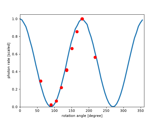
The red circles in the plot mark experimental data from Marshal et al. (2013) (error bars are smaller than plot symbols). In the lab, the distances between sources, mirrors, and detector are much longer than in our setup here. In the simulation, we set up the mirrors to work as if every photon hit with exactly the Brewster angle, while in practice the beam diverges visibly. In the lab, a more parallel beam can be achieved with larger distances between the components. We could change the coordiantes of the mirrors defined above to match the lab setup, but that would make the 3d display, which this example is meant to show-case, less appealing in the limited space of a website.

While not an exact match, this plot in general verifies MARXS polarization calculations to experimental data.

Navigation

Further examples¶

Polarization¶