Define the source in a MARXS run
A “source” in MARXS is anything that sends out X-ray photons. This can be an astrophysical object (such as a star or an AGN, but also a dust cloud that scatters photons from some other direction into our line-of-sight) or a man-made piece of hardware, such as a X-ray tube in the lab or a radioactive calibration source in a satellite. An important distinction in Marxs is weather the source is located at a finite distance (lab source) or so far away that all rays can be treated as parallel (astrophysical source).
For each type of source, we need to specifiy the following properties:
Total flux (or flux density)
Spectrum of photon energies
Polarization
MARXS offers many options to specify the flux, spectrum and polarization that are designed to make common use cases very easy, while allowing for arbitrarily complex models if needed. Examples are given here, the formal specification is written in Source.
In addition, we need to give the location of the source and its size and shape (most of the currently implemented sources are point sources, but additional shapes will be added in the future):
Astrophysical source: Needs coordinates on the sky and a pointing model to translate from sky coordinates to the coordinate system of the satellite. See Specify the sky position of an astrophysical source.
Lab source: Needs x, y, z coordinates in the coordinate system of the experiment as explained in Coordinate system. Lab sources are described in more detail in Specify the position of a laboratory source.
Specify flux, energy and polarization for a source
The source flux, the energy and the polarization of sources are specified in the same way for astrophysical sources and lab sources. We show a few examples here and spell out the full specification below.
Flux
The source flux can just be a number with units:
>>> from marxs.source import PointSource
>>> from astropy.coordinates import SkyCoord
>>> import astropy.units as u
>>> star = PointSource(coords=SkyCoord("23h12m2.3s -3d4m12.3s"), flux=5. / u.s / u.cm**2)
>>> photons = star.generate_photons(20 * u.s)
>>> photons['time'].format='4.1f'
>>> print(photons['time'][:6])
time
 s
----
 0.0
 0.2
 0.4
 0.6
 0.8
 1.0
This will generate 5 counts per second for 20 seconds with an absolutely constant (no Poisson) rate for a default effective area of \(1\;\mathrm{cm}^2\), so the photon list will contain 100 photons.
flux can also be set to a function that takes the total exposure time as input and returns a list of times, one per photon. In the following example we show how to implement a Poisson process where the time intervals between two photons are exponentially distributed with an average rate of 100 events per second (so the average time difference between events is 0.01 s):
>>> from scipy.stats import expon
>>> def poisson_rate(exposuretime):
...     times = expon.rvs(scale=0.01, size=exposuretime.to(u.s).value * 0.01 * 2.)
...     return times[times < exposuretime] * u.s
>>> star = PointSource(coords=SkyCoord(0, 0, unit="deg"), flux=poisson_rate)
Note that this simple implementation is incomplete (it can happen by chance
that it does not generate enough photons). MARXS provides a better implementation
called poisson_process which will generate the appropriate
function automatically given the expected rate:
>>> from marxs.source import poisson_process
>>> star = PointSource(coords=SkyCoord("23h12m2.3s -3d4m12.3s"), flux=poisson_process(100. / u.s / u.cm**2))
Energy
Similarly to the flux, the input for energy can just be a number with a unit, which specifies the energy of a monochromatic source:
>>> FeKalphaline = PointSource(coords=SkyCoord(255., -33., unit="deg"), energy=6.7 * u.keV)
>>> photons = FeKalphaline.generate_photons(5 * u.s)
>>> print(photons['energy'])
energy
 keV
------
   6.7
   6.7
   6.7
   6.7
   6.7
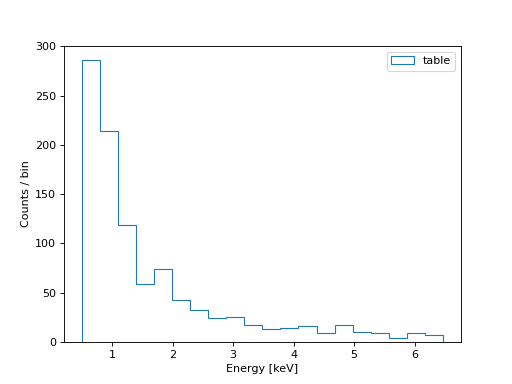
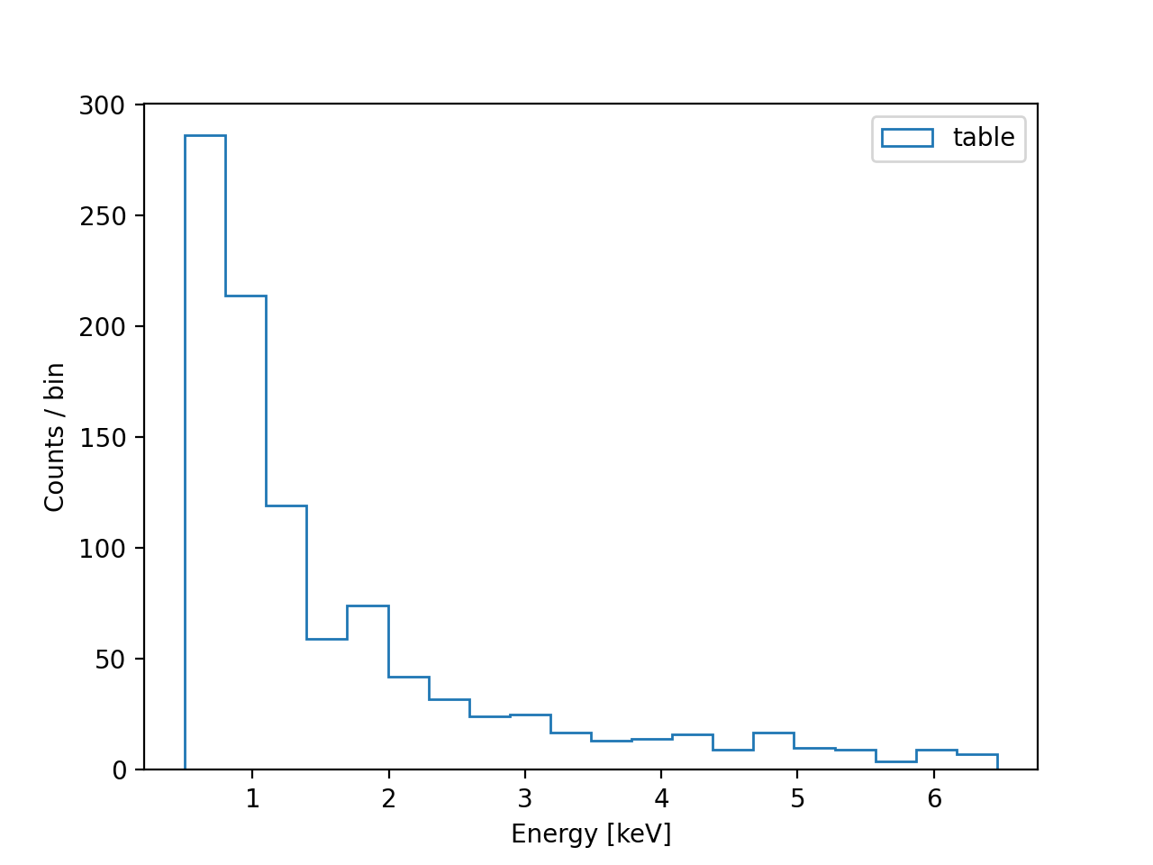
We can also specify a spectrum, by giving binned energy and flux density values. The energy values are taken as the upper egde of the bin; the first value of the flux density array is ignored since the lower bound for this bin is undefined. The format of the spectrum should be a QTable with columns named “energy” and “fluxdensity” (photons/s/area/keV):
import numpy as np
import matplotlib.pyplot as plt
from astropy.table import QTable
import astropy.units as u
from marxs.source import Source
en = np.arange(0.5, 7., .5) * u.keV
fluxperbin = en.value**(-2) / u.s / u.cm**2 / u.keV

# Input as astropy QTable
tablespectrum = QTable([en, fluxperbin], names=['energy', 'fluxdensity'])
s = Source(energy=tablespectrum, name='table')

fig = plt.figure()

photons = s.generate_photons(1e3 * u.s)
plt.hist(photons['energy'], histtype='step', label=s.name, bins=20)

leg = plt.legend()
lab = plt.xlabel('Energy [keV]')
lab = plt.ylabel('Counts / bin')
(Source code, png, hires.png, pdf)

Two helpful hints:
If the input spectrum is in some type of file, e.g. fits or ascii, the
astropy.table.QTableread/write interface offers a convenient way to read it into python:>>> from astropy.table import QTable >>> spectrum = QTable.read('AGNspec.dat', format='ascii') >>> agn = PointSource(coords=SkyCoord("11h11m1s -2d3m2.3s", energy=spectrum)
The normalization of the source flux is always is always given by the
fluxparameter, independent of the normalizion ofspectrum['energy']. If the input is a table and the flux density in that table is in units of photons/s/cm^2/keV, then it is easy to add all that up to set the flux parameter:>>> flux = (spectrum['fluxdensity'][1:] * np.diff(spectrum['energy'])).sum() >>> agn = PointSource(coords=SkyCoord("11h11m1s -2d3m2.3s", energy=spectrum, ... flux=flux)
Lastly, “energy” can be a function that assigns energy values based on the timing of each photon. This allows for time dependent spectra. As an example, we show a function where the photon energy is 0.5 keV for times smaller than 5 s and 2 keV for larger times.
>>> from marxs.source import Source
>>> import numpy as np
>>> def time_dependent_energy(t):
...     t = t.value  # convert quantity to plain numpy array
...     en = np.ones_like(t)
...     en[t <= 5.] = 0.5
...     en[t > 5.] = 2.
...     return en * u.keV
>>> mysource = Source(energy=time_dependent_energy)
>>> photons = mysource.generate_photons(7 * u.s)
>>> print(photons['time', 'energy'])
time energy
 s    keV
---- ------
 0.0    0.5
 1.0    0.5
 2.0    0.5
 3.0    0.5
 4.0    0.5
 5.0    0.5
 6.0    2.0
Polarization
An unpolarized source can be created with polarization=None (this is also
the default). In this case, a random polarization is assigned to every
photon. The other options are very similar to “energy”: Allowed are a constant
angle or a table with columns “angle” and “probabilitydensity”. Here is an example
where most polarizations are randomly oriented, but an orientation around
\(35^{\circ}\) (0.6 in radian) is a lot more likely.
>>> angles = np.array([0., 30., 40., 360]) * u.degree
>>> prob = np.array([1, 1., 8., 1.]) / u.degree
>>> polsource = PointSource(coords=SkyCoord(11., -5.123, unit='deg'), polarization=QTable({'angle': angles, 'probabilitydensity': prob}))
Lastly, if polarization is a function, it will be called with time and energy as parameters allowing for time and energy dependent polarization distributions. The following function returns a 50% polarization fraction in the 6.4 keV Fe florescence line after some polarized feature comes into view at t=1000 s.
>>> def polfunc(time, energy):
...     pol = np.random.uniform(high=2*np.pi, size=len(time))
...     ind = (time > 1000. * u.s) & (energy > 6.3 * u.keV) & (energy < 6.5 * u.keV)
...     # set half of all photons with these conditions to a specific polarization angle
...     pol[ind & (np.random.rand(len(time))> 0.5)] = 1.234
...     return pol * u.rad
>>> polsource = Source(energy=tablespectrum, polarization=polfunc)
Specify the sky position of an astrophysical source
An astrophysical source in marxs must be followed by a pointing model as first optical element that translates the sky coordiantes into the coordinate system of the satellite (see Coordinate system) and an entrace aperture that selects an initial position for each ray (all rays from astrophysical sources are parallel, thus the position of the source on the sky only determines the direction of a photon but not if it hits the left or the right side of a mirror). See Entrance apertures for more details.
The following astrophysical sources are included in marxs:
Sources can be used with the following pointing models:
Specify the position of a laboratory source
Sources in the lab are specified in the same coordinate system used for all other optical elements, see Coordinate system for details.
The following laboratory sources are provided:
Design your own sources and pointing models
The base class for all marxs sources is Source. The only method required for a source is generate_photons. We recommend to look at the implementation of the included sources to see how this is done best.
Reference/API
marxs.source Package
Functions
|
Return a function that generates Poisson distributed times with rate |
Classes
|
Astrophysical source with the shape of a circle or ring. |
|
Simple in-lab point source used with aperture |
|
Transform spacecraft to fixed sky system. |
|
Astrophysical source with a Gaussian brightness profile. |
|
Transform spacecraft to fixed sky system. |
|
In-lab point source |
|
Astrophysical point source. |
|
Base class for sources where photons follow some radial distribution on the sky |
|
Base class for all photons sources. |
|
Astrophysical source with the shape of a circle or ring. |
|
Source shaped like the letter F. |