Running MARXS at a glance

A MARXS simulation can be customized in many different ways to adapt to different instruments and science questions. Therefore, some classes support quite complex input. Before discussing all options in detail, we want to present a complete MARX run with typical parameters here.

Our question is the following: We will simulate an observation with the Chandra X-ray observatory. Chandra dithers its pointing on the sky. We want to know what pattern this dither makes on the detector for a fairly short observation. MARXS includes a simplified description of the Chandra X-ray observatory in the marxs.missions module.

Creating a source

First, we need to set up a point sources with a spectrum and a total flux. We have to set the positions of our sources as an astropy.coordinates.SkyCoord:

>>> from astropy.coordinates import SkyCoord
>>> ngc1313_X1 = SkyCoord("3h18m19.99s -66d29m10.97s")

In many cases, the spectrum of the sources will come from a table that is generated from a simulation or from a table written by a program such as XSPEC or Sherpa. MARXS sources accept a wide range of input formats (see Specify flux, energy and polarization for a source) including plain numpy arrays for an energy grid and a flux density grid in photons/s/cm**2/bin. Our source here has a simple power-low spectrum. We ignore extinction for the moment which would significantly reduce the flux we observe in the soft band.

>>> import numpy as np
>>> import astropy.units as u
>>> from astropy.table import QTable
>>> energies = np.arange(.3, 8., .01) * u.keV
>>> spectrum1 = 6.3e-4 * energies.value**(-1.9) / u.s / u.cm**2 / u.keV

Marxs sources have separate parameters for the energy (shape of the spectrum) and the flux (normalization of the spectrum and temporal distribution). In many cases we want to apply the same spectrum with different normalizations to different sources, so it is useful to separate the shape of the spectrum and the total flux. We simulate a source that is constant in time, so the photon arrival times will just be Poisson distributed. In this case, the input spectrum is already properly normalized, so we just sum it all up to to get the total flux. Note that MARXS interprets the energy array as the upper energy bound for each bin. The lower energy bound is gives as the upper energy bound from the previous bin. This leaves the lower bound of the first bin undefined and thus we do not include it in the sum.

>>> from marxs.source import poisson_process
>>> flux1 = (spectrum1[1:] * np.diff(energies)).sum()
>>> flux1 = poisson_process(flux1)

The last thing that the source needs to know is how large the geometric opening of the telescope is, so that the right number of photons are generated. So, we create an instance of the Chandra mirror with the parameter file included in the MARXS distribution:

>>> from marxs.missions import chandra
>>> aperture = chandra.Aperture()

Now, can can finally create our source:

>>> from marxs.source import PointSource
>>> src1 = PointSource(coords=ngc1313_X1, energy=QTable({'energy': energies, 'fluxdensity': spectrum1}),
...                    flux=flux1, geomarea=aperture.area)

See Define the source in a MARXS run for more details.

Set up observation and instrument configuration

We need to specify the pointing direction and the roll angle (if different from 0):

>>> pointing = chandra.LissajousDither(coords=ngc1313_X1)

and also set up the instrument components. The entrace aperture was already initialized above, and the rest is easy because it is already included in MARXS (but keep in mind that the Chandra model used here includes only the geometry. It leaves out many important effects which require aceess to CALDB data, such as ACIS contamination, order probabilities for gratings etc. Use classic marx to simulate Chandra data for real.)

>>> hrma = chandra.HRMA()
>>> acis = chandra.ACIS(chips=[4,5,6,7,8,9], aimpoint=chandra.AIMPOINTS['ACIS-S'])

That was easy!

If you are simulating an instrument that is not part pf the MARXS package itself you can either specify everything yourself (see Optical elements that make up an instrument for more details) or use files provided, e.g. by the instrument team. In that case, you have probably also received more detailed instructions on how to use these files.

Run the simulation

In MARXS, a source generates a photon table and all following elements process this photon table by changing values in a column or adding new columns. Thus, we can stop and inspect the photons after every step (e.g. to look at their position right after they exit the mirror) or just execute all steps in a row:

>>> photons = src1.generate_photons(5 * u.ks)
>>> photons = pointing(photons)
>>> photons = aperture(photons)
>>> photons = hrma(photons)
>>> photons = acis(photons)

Look at simulation results

In MARXS, if you want to know the number of photons that are expected to be detected, you select the photons in the output list that hit the detector and then add up all the probabilities:

>>> ind = photons['CCD_ID'] > 0
>>> 'Expected number of photons: {}'.format(photons['probability'][ind].sum()) 
'Expected number of photons: ...'

If, instead, you are looking for a list of detected photons which has the same noise levels, you need to draw a subset of events from the photon list:

>>> pobs = photons[photons['probability'] < np.random.uniform(len(photons))]

For more details on the MARXS output see MARXS Output.

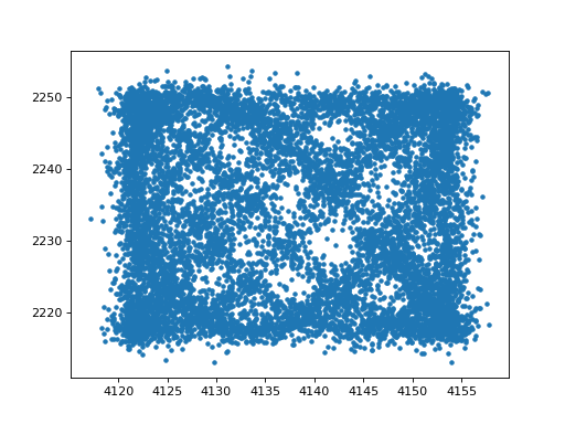
We can now look at the distribution of photons on the detector:

>>> from matplotlib import pyplot as plt
>>> line = plt.plot(photons['tdetx'], photons['tdety'], '.')

The plot clearly shows the dither pattern on the sky.

(Source code, png, hires.png, pdf)

For more details on visualization see Visualize results.